Making Route Using Open Trip Planner (OTP) and Open Source Routing Machine (OSRM)

In this article, we’re trying to make route using QGis, R, Open Trip Planner (OTP) and Open Source Routing Machine (OSRM). The cases that we’re trying to do are:

• Activate the OTP Server in the Local Host
• Create a Point to Point Route using OTP and R
• Define the Service Area using OTP and R
• Route Analysis using OSRM and R

Open Trip Planner (OTP) is a family of the open source software projects that provide passenger information and transportation network analysis services. The core server-side Java component finds itineraries combining transit, pedestrian, bicycle, and car segments through networks built from widely available, open standard OpenStreetMap and GTFS data. This service can be accessed directly via its web API or using a range of Javascript client libraries, including modern reactive modular components targeting mobile platforms.

Open Trip Planner’s server can be located in our local host, so we can freely access and modify the data.

Case 1 : Activate the OTP Server in the Local Host

The first step before we activate the server is we should install the local server for Open Trip Planner. After that, we should put the GTFS and pbf data in our current directory folder. In this case we use Singapore GTFS data.

GTFS (General Transit Feed Specification) is the data of specification that allows public transit agencies to publish their transit data in a format that can be consumed by a wide variety of software applications. Today, the GTFS data format is used by thousands of public transport providers.

GTFS is split into a static component that contains schedule, fare, and geographic transit information and a real-time component that contains arrival predictions, vehicle positions and service advisories.

To start the installation process of the OTP server, we should put the otp.jar file in the directory folder. The otp.jar can be downloaded uses this step. After that, change the directory on command prompt, with the directory that we have saved the otp.jar file. Next, activate the otp.jar by using this code in command prompt:

java -Xmx2G -jar otp.jar --build graphs/current -–analyst

the Graph.obj file will appear in the directory, and for the next step, we can activate the server using this code in command prompt:

java -Xmx2G -jar otp.jar --router current --graphs graphs --server --analyst --port 8801 --securePort 8802

and then we can check the server on our browser :

http://localhost:8801/

Case 2: Create a Point to Point Route using R

The first step for making point to point route is installing the “opentripplanner” package in R. We can use this code for installing and calling the package:

remotes::install_github("ropensci/opentripplanner")
library(opentripplanner)

After that, connect the local server of OTP with R, by using this code:

otpcon <- otp_connect(hostname = "localhost", router = "default", port = 8801)

Let’s making a route!!!

For the example we choose the longitude and latitude point from the Changi to Merlion : (103.98602, 1.35008) and (103.85359, 1.28685). And then we’re trying to make a route using this code below:

route <- otp_plan(otpcon,
                  fromPlace = c(103.98602,1.35008),
                  toPlace = c(103.85359,1.28685))
#Install Tmap Packages for Plotting the Route 
install.packages("tmap")
library(sf)
library(tmap)
tmap_mode("view") 
qtm(route)
st_write(route, "route.shp")
library(sf)
library(tmap)
tmap_mode("view") 
qtm(route, lines.lwd = 3, lines.col = "red")

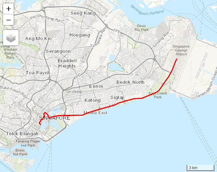
We can visualize the route.shp’s file that already made in R, using QGis by adding the vector layer of that file:

The figure above is the mapping result of the route, from point (103.98602, 1.35008) to point (103.85359, 1.28685) that we have made using Singapore GTFS file, R and visualize it using QGis.

Case 3: Define the Service Area

For the Case 3, we’re gonna make how far isochrone that will be made from Changi airport.

An isochrone map in geography and urban planning is a map that depicts the area accessible from a point within a certain time threshold. An isochrone (iso = equal, chrone = time) is defined as “a line drawn on a map connecting points at which something occurs or arrives at the same time”. In hydrology and transportation planning isochrone maps are commonly used to depict areas of equal travel time.

Before we start to make the service area, we should call the library that we need for defining the service area, by using this code:

library(httr)
library(sp)
library(tidyverse)
library(leaflet)
library(geojsonio)

and then we call the API by using this code:

changi <- GET(
  "http://localhost:8801/otp/routers/current/isochrone",
  query = list(
    toPlace = "1.35600,103.985",
    fromPlace = "1.35600,103.985",
    arriveBy = TRUE,
    mode = "CAR", # modes we want the route planner to use
    date = "11-21-2020",
    time= "12:00am",
    maxWalkDistance = 1600, # in metres
    walkReluctance = 5,
    minTransferTime = 600, # in secs (allow 10 minutes)
    cutoffSec = 900,
    cutoffSec = 1800,
    cutoffSec = 2700,
    cutoffSec = 3600,
    cutoffSec = 4500,
    cutoffSec = 5400
  )
)

after that, we can use this code for making or defining the service area of the Changi airport:

changi <- content(changi, as = "text", encoding = "UTF-8") 
write(changi, file = "changi.geojson")
iso <- geojsonio::geojson_read("changi.geojson",
                               what = "sp")
pal=c('cyan','gold','tomato','red')
m <- leaflet(iso) %>%
     setView(lng = 103.8198, lat = 1.3521, zoom = 11) %>%
     addProviderTiles(providers$CartoDB.DarkMatter, options =     
     providerTileOptions(opacity = 0.8)) %>%
     addPolygons(stroke = TRUE, weight=0.5, smoothFactor = 0.3,
     color="black", fillOpacity = 0.1,fillColor =pal ) %>%
  addLegend(position="bottomleft",colors=rev(c("lightskyblue","greenyellow","gold","tomato")), labels=rev(c("60 min","45 min","30 min","15 min")), opacity = 0.6, title="Travel Time with Public Transport")
m

The Result of the Changi’s Isochrone

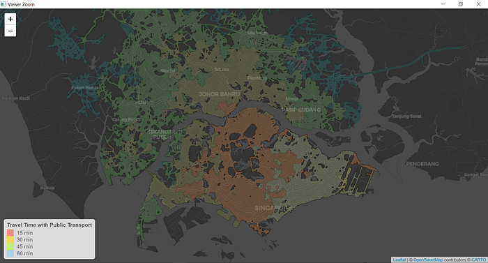
From the output figure above we can see the travel time with public transport from Changi. The red color shows the travel time with a duration of 15 minutes, the orange, green and blue color shows the travel time with a duration of 30 minutes, 45 minutes and 60 minutes.

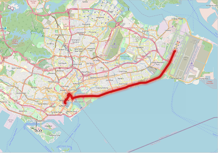
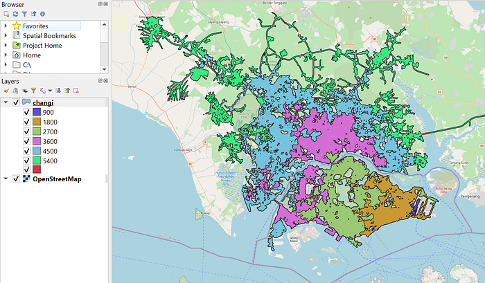
If we add the geojson file in QGis, and changes the classify the categories by time, we can get this map:

Case 4 : Route Analysis using OSRM and R

In this case, we’re going to make route analysis by distance and duration using OSRM and R.

The Open Source Routing Machine or OSRM is a C++ implementation of a high-performance routing engine for the shortest paths in road networks. It combines sophisticated routing algorithms with the open and free road network data of the OpenStreetMap (OSM) project. Shortest path computation on a continental sized network can take up to several seconds if it is done without a so-called speedup-technique. OSRM uses an implementation of contraction hierarchies and is able to compute and output a shortest path between any origin and destination within a few milliseconds, whereby the pure route computation takes much less time.

Since it is designed with OpenStreetMap compatibility in mind, OSM data files can be easily imported.

We can access the OSRM using R by installing the package using this code:

install.packages("osrm")
library(osrm)

In this case we use the default dataset from the osrm packages. The dataset contain the 100 drugstore location in Berlin. We can use this code below for making the route between the drugstore that we’ll choose

# Load data
data("berlin")
library(sf)
# Travel Path Between Points
route1 <- osrmRoute(src = apotheke.sf[1, ], dst = apotheke.df[11, ], returnclass="sf") # Travel path between points excluding motorways
# Visualize the plot
library(tmap)
tmap_mode("view") 
qtm(route1, lines.lwd = 3, lines.col = "red")

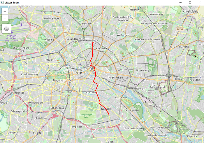
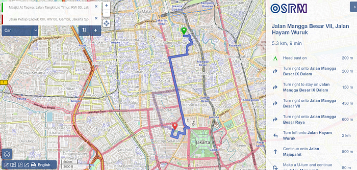
From the figure above, finally we got the route from the apotekhe 1 to the apotheke 2. For the next step we’re trying to know the duration and the distance between two apotekhe by using this code:

# Return Only Duration and Distance
route2 <- osrmRoute(src = apotheke.sf[1, ], dst = apotheke.df[11, ], overview = FALSE)
route2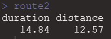

And if we only have the point of the location, we can calculate the duration and the distance also by using this code:

# Using Only Coordinates
route3 <- osrmRoute(src = c(13.412, 52.502),
                    dst = c(13.455, 52.580), returnclass = "sf")
tmap_mode("view") 
qtm(route3, lines.lwd = 3, lines.col = "red")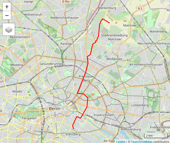

Map showing a route from many points

# Using via points
osrmTable
pts <- structure( list(x = c(13.32500, 13.30688, 13.30519, 13.31025,
13.4721, 13.56651, 13.55303, 13.37263, 13.50919, 13.5682), y = c(52.40566, 52.44491, 52.52084, 52.59318, 52.61063, 52.55317,
52.50186, 52.49468, 52.46441, 52.39669)), class = "data.frame", row.names = c(NA, -10L))
route4 <- osrmRoute(loc = pts, returnclass = "sf")
tmap_mode("view") 
qtm(route4, lines.lwd = 3, lines.col = "red")

Map showing a route from many points

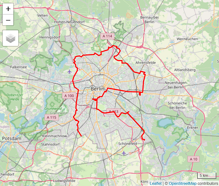
As you can see we have sucessfully made a route consist of two points and many points using R and OSRM.

Finally!! We have succcessfully activated the OTP Server in the Local Host, created a Point to Point Route using OTP and R, defined the service area using OTP and made route analysis using OSRM and R. Hopefully this article is useful and thanks for reading!

References:

e-Workshop — Analisis Jaringan dan Rute Transportasi Multimoda dengan R dan QGIS, Ma ChungUniversity

OpenTripPlanner

Project OSRM